Complexity and optimization
In the general protocol, the number of reference pairwise comparisons scales with how many neighbors each node has—but who is adjacent to whom is left to the implementer.
If each node only has O(1) neighbors, work stays O(n) in n nodes. If the graph is fully connected—every node neighbors every other—the count of edges (hence comparisons) is quadratic, O(n²).
Complete graphs and
For |V| = 2 or 3, even a complete graph is tiny: 1 or 3 reference pairwise comparisons respectively, so complexity is not a practical concern yet.
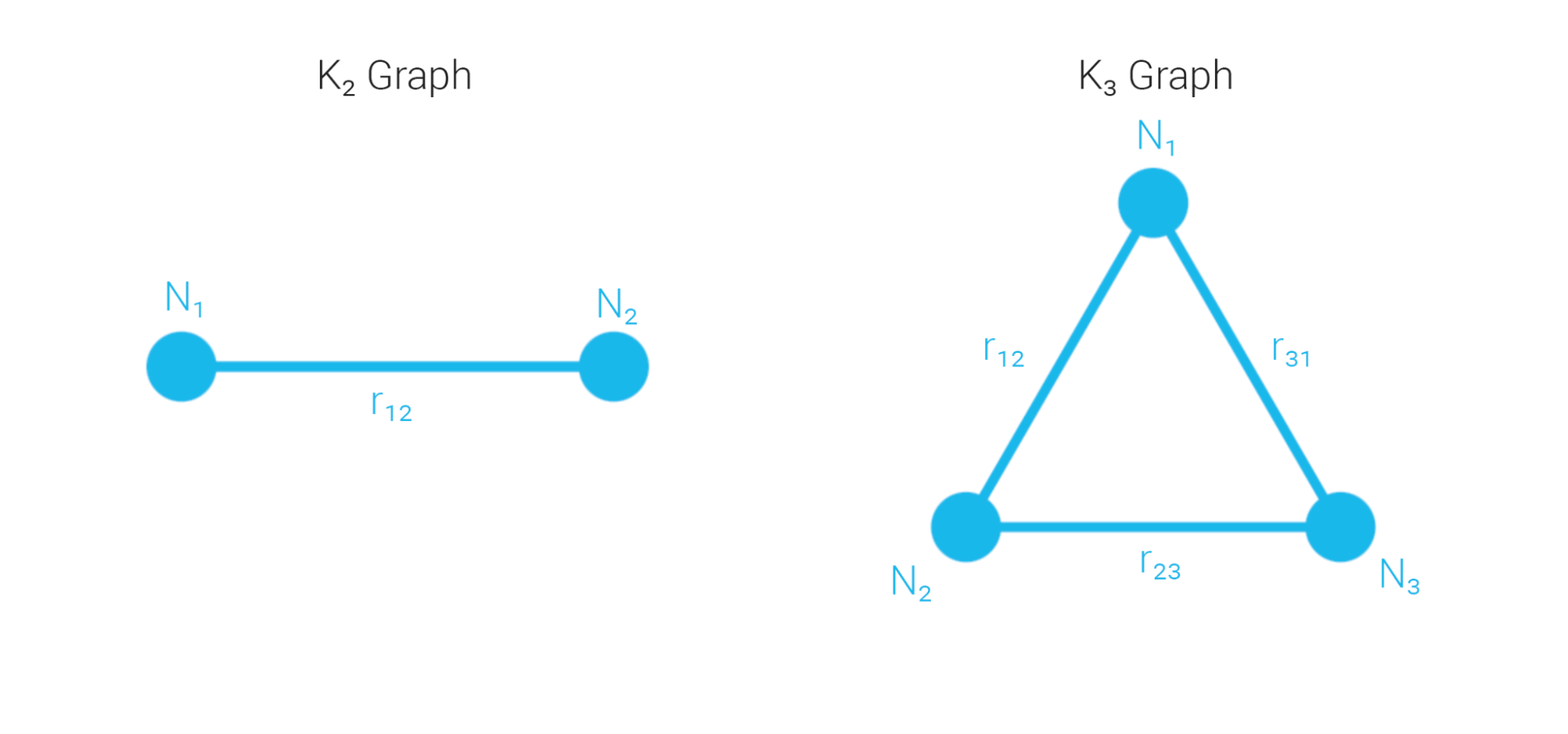
Complete graphs with
Beyond , the edge count of a clique keeps growing quadratically.
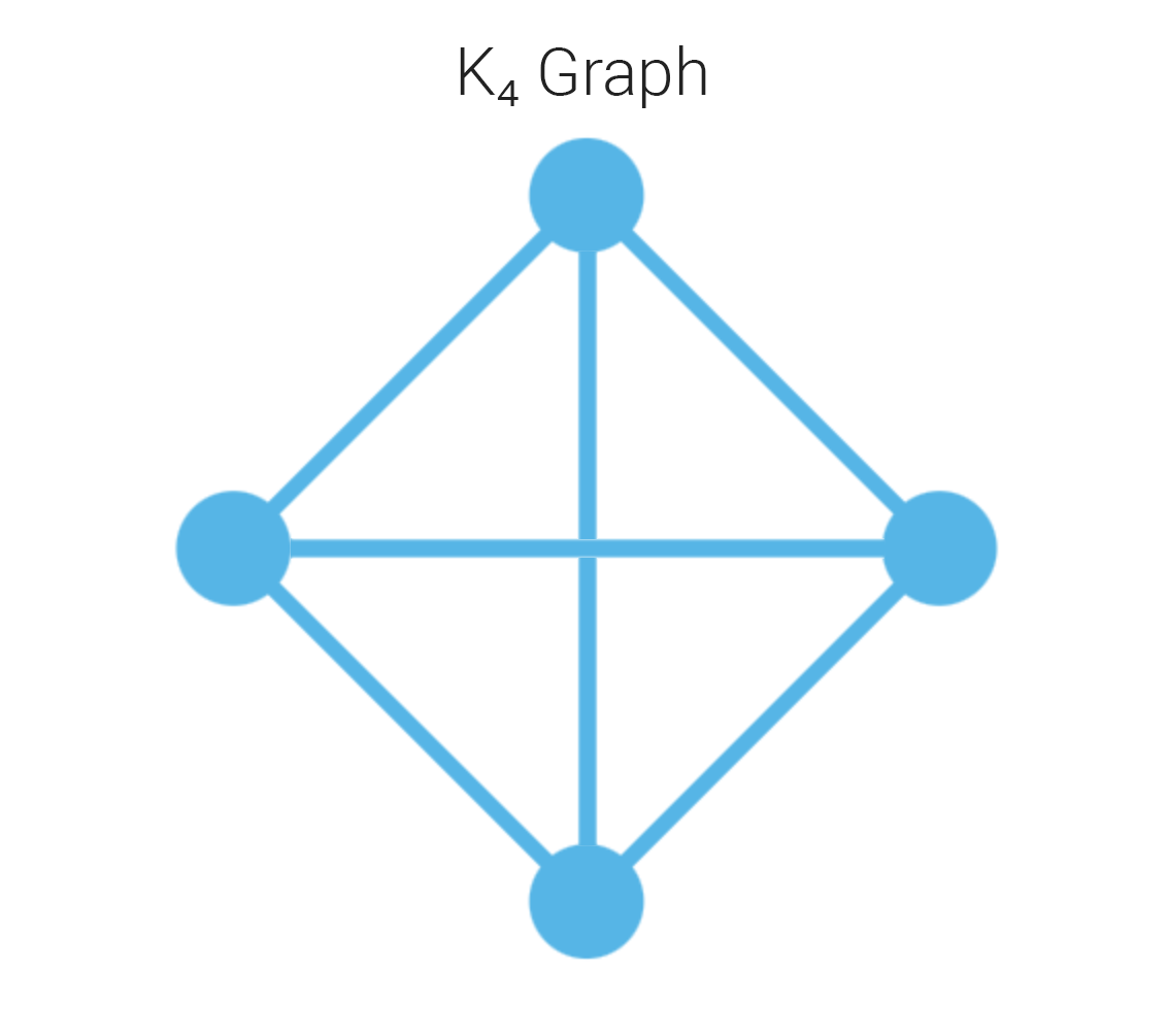
with four vertices and six edges (reference export; prose in the source names this graph explicitly).
For a complete graph on n vertices, the number of edges is
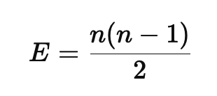
With more than three nodes, fully connected CRPC graphs become expensive fast—each edge also implies two reciprocal attestations, so stored comparison data is 2 × |E|.
Note: Multiply reference comparisons (edges) by two to get the number of published pairwise attestations.
Ring topology
The usual sparse choice is a ring: each node has at most two neighbors. Reference comparisons then scale linearly with n while still yielding useful per-node attestations.
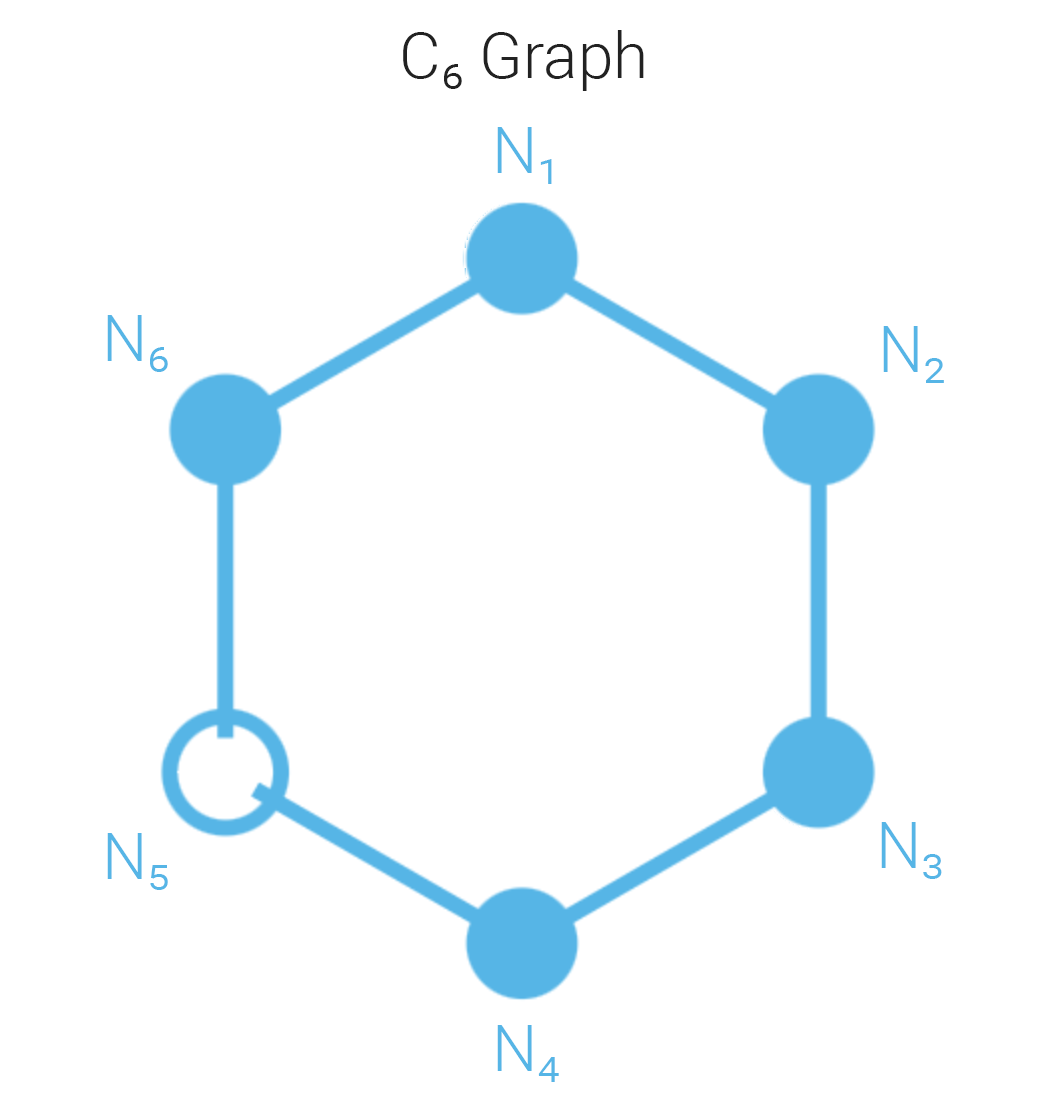
In a example, five nodes may pass local checks while one fails—illustrating how more participants make disputes easier to surface.
We suggest a minimum of three nodes in practice so that, if one node disputes, two others still contribute independent signal.
Complete graphs: comparisons grow as Θ(n²); simple cycles: Θ(n) edges, times two for reciprocity—so dense topologies blow up much faster.
| Nodes | Edges: complete | Edges: cycle |
|---|---|---|
| 2 | 1 | 1 |
| 3 | 3 | 3 |
| 4 | 6 | 4 |
| 5 | 10 | 5 |
| 6 | 15 | 6 |
| 7 | 21 | 7 |
| 8 | 28 | 8 |
Solving the drift problem
For rings with |V| ≥ 4, local thresholds can hide global inconsistency: each edge may look fine while a non-edge pair (e.g. opposite on the ring) would violate ε if measured directly. Call that accumulated gap drift.
Example on
Take nodes with scalar results:
Every measured adjacent difference is ≤ 0.1 < 0.15, so all on edges. Yet —unmeasured drift the naive ring never sees.
Fully connecting the graph would catch that but reintroduces O(n²) edges.
Local vs global ε
Split the budget: let be the true tolerance you care about, and set a stricter per-edge tolerance derived from n.
Use
On a cycle, the worst-case hop distance between two nodes is about ⌊n/2⌋; if each edge obeys an L-Lipschitz-style bound with , then diametrically opposite values are bounded by roughly . (The write-up ties this to choosing so unmeasured pairs stay below without a clique.)
That lets you keep linear edge count while implicitly controlling non-edges, at the cost of tighter per-edge thresholds as n grows.
Demonstration: catching unacceptable drift
Reuse the example with :
Now —the first edge fails the stricter local rule, so we reject the configuration before trusting unmeasured pairs such as .
Even without explicitly computing , we already know would have been a problem; gives a linear-time certificate that would have been invisible under a single naive on the ring alone.
In practice, tightening buys much of the safety of a dense graph while keeping sparse topology.