Quantitative pairwise comparisons

The CRPC protocol is chiefly focused on pairwise comparisons whose results can be measured in a quantitative format—for example, a floating-point number representing the similarity between two pieces of text.

The sections below walk through two concrete examples, derive the general format of a quantitative pairwise comparison, and then extend the idea to networks and adversarial settings.

Example 1: Semantic Textual Similarity (STS)

Semantic Textual Similarity (STS) is a method of determining, regardless of syntax or particular wording, how similar two pieces of written text might be.

Consider the example of @0xsmallbrain ’s natural language prediction market for tomorrow’s headlines: tmr.news .

That site lets users predict the next day’s New York Times headline on a decentralized market, using a cosine similarity algorithm that compares each user’s headline to the actual headline (revealed a day later) to determine payouts.

Screenshot of tmr.news headline prediction market — tmr.news by 0xsmallbrain (screenshot, 2024-09-21).

Consider the following headlines and their similarity scores in the prediction market for September 21st, 2024:

$S_1$ = “Senior Hezbollah Leader is Killed in Beirut in Israeli Airstrike” (actual)
$S_2$ = “Senior Hezbollah Leader Killed by Israeli Airstrike in Lebanon” (0.95)
$S_3$ = “Israel Targets Senior Hezbollah Leader in Beirut Airstrike” (0.87)

The site documents that “Scores are calculated using sentence embeddings (sic), specifically using cosine similarity and OpenAI’s text-embeddings-3-large model with dimension 768.”

After each sentence is converted to a vector of embedded tokens (numerical representations) using OpenAI’s text-embeddings-3-large model, cosine similarity is applied to each vector to produce a score between 0 and 1, where 1 means “most alike.”

For reference, a vector of embeddings for $S_1$ begins like: [-0.009729066863656044, 0.010178100317716599, -0.002148742089048028, …].

The usual form of the cosine similarity of two vectors A and B is:

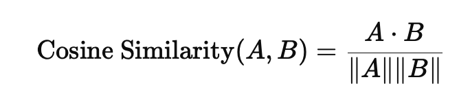
\cos(\theta) = \frac{\mathbf{A} \cdot \mathbf{B}}{\|\mathbf{A}\| \|\mathbf{B}\|} = \frac{\sum_{i=1}^{n} A_i B_i}{\sqrt{\sum_{i=1}^{n} A_i^2}\,\sqrt{\sum_{i=1}^{n} B_i^2}}

Embedding vector fragment and cosine similarity formula as in the reference write-up — Embedding vector example and cosine similarity form (reference export).

For the headline embeddings $S_1$ , $S_2$ , $S_3$ :

\frac{\mathbf{s}_1 \cdot \mathbf{s}_2}{\|\mathbf{s}_1\| \|\mathbf{s}_2\|} = 0.95, \qquad \frac{\mathbf{s}_1 \cdot \mathbf{s}_3}{\|\mathbf{s}_1\| \|\mathbf{s}_3\|} = 0.87

Thus the pairwise comparisons between $S_1$ and $S_2$ , then $S_1$ and $S_3$ , are the cosine similarities of their respective embedding vectors (each a scalar in $[0, 1]$ for comparable, length-normalized embeddings).

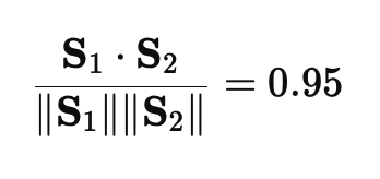
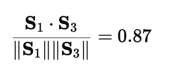
Pairwise cosine similarity scores between headline embeddings — Pairwise comparisons among $S_1$ , $S_2$ , and $S_3$ (reference export; two-part figure).

Pairwise scores continued from the reference export — Pairwise comparisons among $S_1$ , $S_2$ , and $S_3$ (reference export; two-part figure).

The winner of the prediction market that day was $S_2$ , with a score of 0.95 over the nearest competitor’s 0.87—showing how rich text can still be reduced to a quantitative pairwise comparison.

Note: Cosine similarity for STS does not catch every failure mode—for example, semantic inversions such as “is” vs “isn’t.”

Example 2: Image similarity

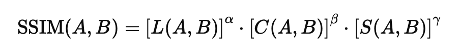
Mathematical ways to compare images, such as the Structural Similarity Index (SSIM), are well established.

Suppose a smart contract (an NFT generator for an on-chain game) wants a new potion image. It issues a request to two nodes in a known-good “AI Drawing Service Pool.”

Node A and Node B each render an image from this prompt:

(masterpiece, highest quality), a potion bottle filled with glowing purple liquid, purple theme, video game art, 3D rendering, volumetric lighting, fantasy, simple background

Node A’s result	Node B’s result

Neither image is identical—we did not fix seeds, steps, or speed optimizations such as xformers—yet either image can be acceptable as a “purple potion” NFT.

A smart contract cannot do a human-like visual review. A numerical pipeline using SSIM (e.g. via oracles) can compare the two renders. SSIM combines luminance (L), contrast (C), and structure (S):

\mathrm{SSIM}(A, B) = \bigl[L(A, B)\bigr]^{\alpha} \bigl[C(A, B)\bigr]^{\beta} \bigl[S(A, B)\bigr]^{\gamma}

Difference maps can be visualized between images A and B.

SSIM-based comparison pipeline for oracles — SSIM-style comparison concept (reference export).

Luminance, contrast, and structure components and difference-style visualization between two images — Luminance, contrast, structure, and visual differences between images A and B (reference export).

Mismatched potion render from an incorrect prompt — Example where one node used a wrong prompt (green bottle / ivy); SSIM drops vs acceptable purple potions (reference export).

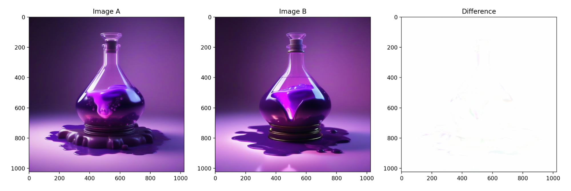
For the two acceptable purple potions, SSIM can land near 0.99902838508614.

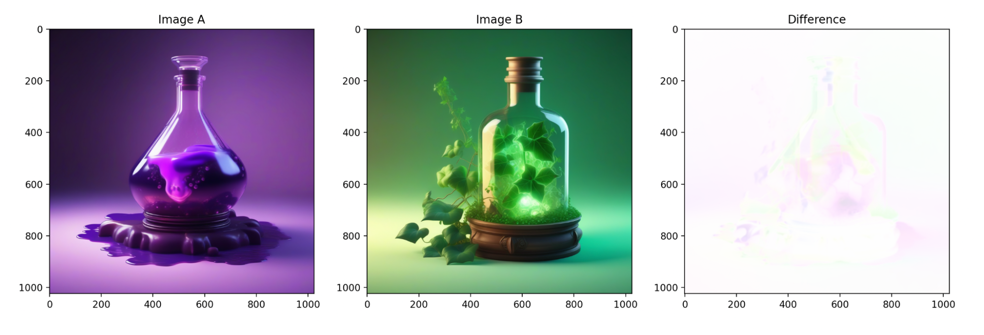
If one node accidentally used a wrong prompt (e.g. a cached green bottle with ivy), the visuals diverge and SSIM drops—for example to 0.9877919695121076.

Note: You can increase sensitivity (e.g. emphasize structure) by tuning SSIM’s $\gamma$ parameter, or by choosing a stronger perceptual similarity metric.

Acceptable error thresholds

The gap between an acceptable score and an unacceptable one can look tiny (here, about 0.011236415574032), but fuzzy or non-deterministic work needs an explicit acceptable error threshold.

Let $\epsilon$ (epsilon) be that threshold: the comparison difference $\delta$ (delta) should satisfy $\delta < \epsilon$ when similarity is the goal (smaller $\delta$ means “closer match”).

In the purple-potion example, you might set $\epsilon = 0.001$ . The $\delta$ between the two good images was 0.00097161491386, which is within the acceptable range.

Example 3: Rolling dice and randomness

You can invert the relationship: require pairwise comparisons to be above a threshold so outputs are sufficiently different. That fits pseudo-randomness for web3 games and autonomous worlds.

Many tools exist (VRFs, MPC, RANDAO, and others). CRPC can still help deliver usable pseudo-random values on demand—for example, within the next block after a request.

A possible Ethereum-shaped sketch:

Three nodes are tasked with a pseudo-random number in a given range.
Each node runs a PRNG (e.g. Mersenne Twister) with a seed mixing the block hash and the node id (to discourage caching old useful outputs).
Each node advances the PRNG state by a fixed number of discarded draws (not wall-clock time), then outputs a value.
CRPC secures outputs and pairwise comparisons on-chain.
The contract checks that results differ enough: $\delta_{ij} \geq \epsilon$ (pairwise gaps across nodes).
The contract then selects which node’s value to use (e.g. with the next block hash).

Observers can replay the PRNG steps and report cheating. Because the contract might not pick a lying node’s value, incentives skew toward honesty; full incentive design belongs to a larger consensus layer.

CRPC-style randomness also keeps flexibility in distribution and range—Gaussian vs uniform, and so on—beyond what some VRF / RANDAO-style APIs expose.

General form of pairwise comparisons in a network

Formalize pairwise comparisons on a graph: nodes compute results independently; small differences from noise or benign variation should fall within $\epsilon$ .

Definitions:

$\Phi$ — the result of a node’s work.
$\delta$ — the difference between two nodes’ results (how you instantiate this depends on the metric: embedding distance, $1 - \text{SSIM}$ , etc.).
$\epsilon$ — the agreed acceptable error threshold.

Let node $N_i$ produce $\Phi_i$ . The pairwise comparison along an edge between $N_i$ and $N_j$ is $\delta_{ij}$ . A common choice for scalar outputs is the absolute difference:

\delta_{ij} = \lvert \Phi_i - \Phi_j \rvert

Notation for Phi_i, Phi_j, and pairwise comparison delta_ij — $\Phi_i$ , $\Phi_j$ , and $\delta_{ij}$ (reference export).

An acceptable comparison (in the “similar enough” regime) satisfies:

\delta_{ij} < \epsilon

Acceptable comparison defined with threshold epsilon — Acceptable comparison vs threshold $\epsilon$ (reference export).

A network of n nodes is a graph with $\lvert V \rvert \geq 2$ . A directed edge value can be identified with the measured comparison when you use absolute difference on scalars:

e_{ij} = \delta_{ij} = \lvert \Phi_i - \Phi_j \rvert

Graph with edges as pairwise comparisons between nodes — Network as a graph; edges $e_{ij}$ as pairwise comparisons (reference export).

That graph view supports reference pairwise comparisons $r_{ij}$ : the value two honest, faultless nodes would publish on the same edge if they agreed. When reciprocals match, define $r_{ij}$ from the common edge value; otherwise the reference is undefined:

r_{ij} = \begin{cases} e_{ij}, & \text{if } e_{ij} = e_{ji} \\[0.35em] \text{undefined}, & \text{if } e_{ij} \neq e_{ji} \end{cases}

Reference pairwise comparisons r_ij under honest conditions — Reference comparisons $r_{ij}$ when nodes agree (reference export).

Pairwise comparisons under decentralized conditions

CRPC targets settings where nodes may be faulty or malicious, producing unacceptable comparisons or disagreeing on what the reference comparison along an edge should be.

In decentralization there is no trusted third party that knows the true $r_{ij}$ by inspecting $\Phi_i$ and $\Phi_j$ directly.

Instead, each node compares its output to its neighbor’s. For every undirected edge you get two published comparisons— $\delta_{ij}$ and $\delta_{ji}$ —so the requester can validate consistency.

Example setup

Take two nodes and arbitrary work W:

$N_1$ computes $\Phi_1 = 100$
$N_2$ computes $\Phi_2 = 99$
Threshold $\epsilon = 2$
The nodes form a complete graph $K_2$

We still do not know the “true” $\Phi$ for W; we use multiple nodes to test consistency or surface disputes so the requester can decide whom to trust.

From here we can state requirements CRPC must meet to be usefully trust-minimized.

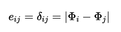
Case 1: Both nodes honest and faultless

Case 1: both nodes honest; same reported edge difference — Case 1: both nodes honest and faultless (reference export).

Each node compares honestly; both publish the same edge value, so the mutual reference comparison is $r_{12} = 1$ (here, $\lvert 100 - 99 \rvert$ ). That mutual agreement supports treating the edge as consistent.

Since $r_{12} < \epsilon$ (here $1 < 2$ ), the comparison is acceptable under the threshold—no fault signal from this edge alone.

Note: Both nodes can still be wrong together in a way this edge does not expose; the document discusses that further elsewhere.

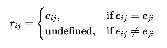
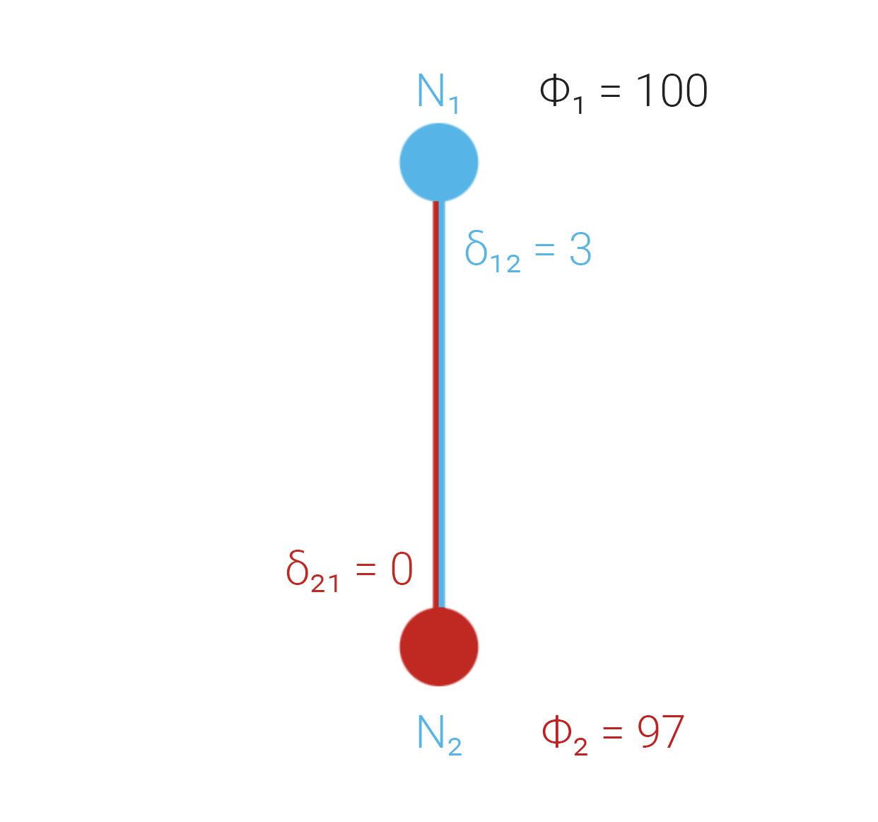
Case 2: One node faulty but honest

Case 2: faulty but honest reporting; reciprocal comparisons still match — Case 2: one node faulty but honest— $\Phi_2$ diverges; both still report the same directed differences (reference export).

Suppose $\Phi_2 = 97$ so $\lvert \Phi_1 - \Phi_2 \rvert = 3$ while $\epsilon = 2$ . Honest reporting keeps $\delta_{12} = \delta_{21} = 3$ , so you can compare $r_{12}$ to $\epsilon$ .

Because 3 > 2, the requester should not treat the outputs as mutually consistent: there is an active dispute. Resolving it belongs to a mechanism above CRPC (e.g. Byzantine Risk Tolerance, BRT).

Note: With only two nodes you cannot tell which side is wrong; $\Phi_1 = 100$ might be the bug. Adding nodes generally improves the chance of catching inconsistencies.

Case 3: One node faulty and dishonest

Case 3: one node reports delta 3, the other falsely reports 0 — Case 3: $N_1$ reports difference 3; $N_2$ falsely reports 0 (reference export).

$N_1$ honestly reports 3 between $\Phi_1$ and $\Phi_2$ . $N_2$ lies and broadcasts 0, as if it matched $N_1$ .

When the work itself is too hard to verify directly, the requester leans on pairwise comparison attestations. If only one side ever spoke, the other could lie unchecked.

So both nodes must separately attest to the difference each computed—even when an honest world would make those values equal.

The diagrams below mirror the TikZ cases in the appendix (graphics section).